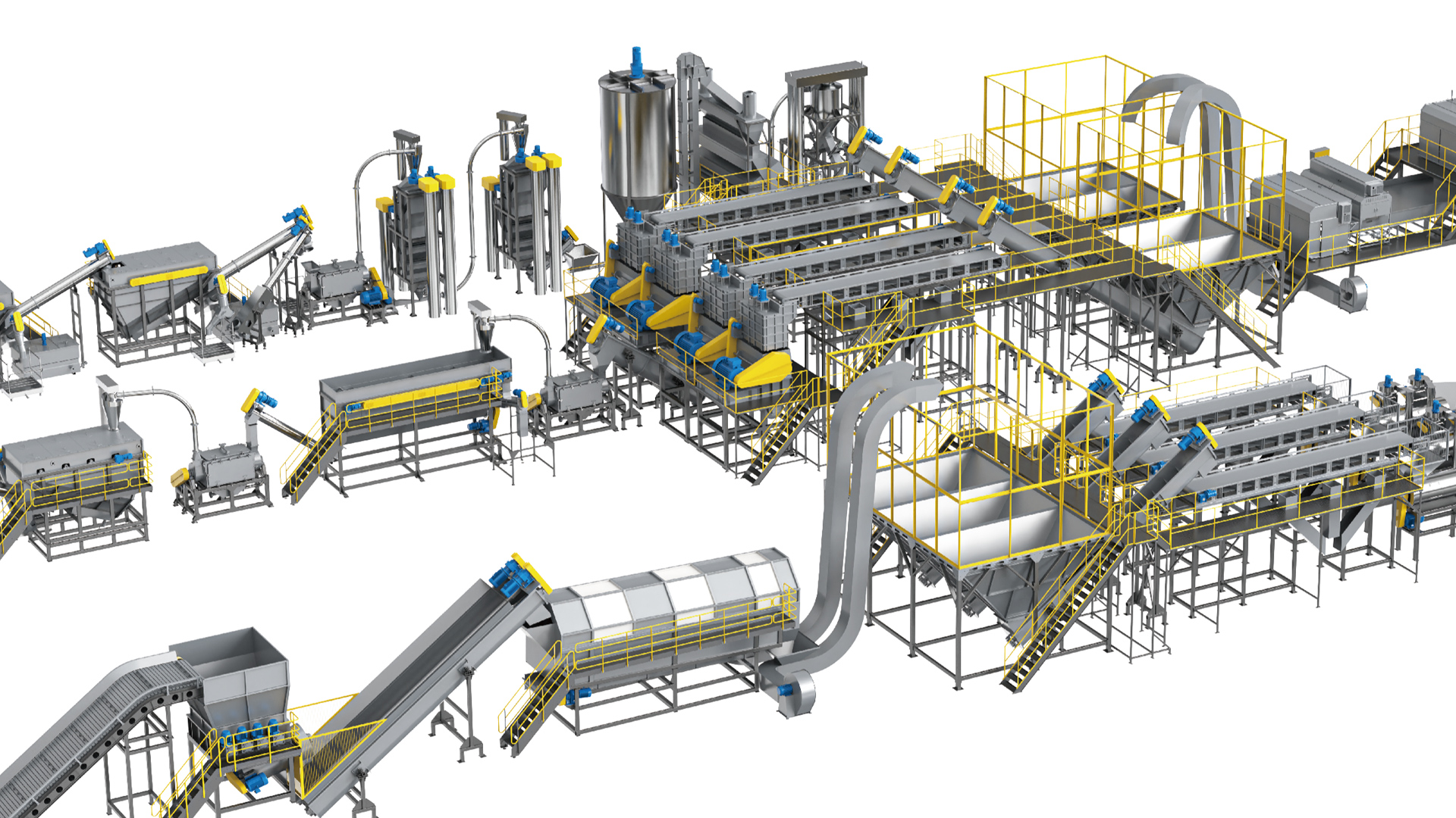

Calculating the ROI of a custom plastic recycling washing line is an exercise in physics before it is an exercise in finance. Every unit of return the plant will ever generate passes first through a mass balance, a utility balance and an availability figure — and those three physical realities are decided during equipment specification, not during the budgeting meeting. Investors who begin with a capital figure and work backwards toward a payback period almost always produce a model that looks defensible and fails in operation. Investors who begin with tonnes per hour, yield percentage, kilowatt-hours per tonne and cubic metres per tonne produce a model that survives contact with a real feedstock stream.
This guide sets out a complete, currency-neutral framework for building that model. Every cost is expressed as a relative tier — Low, Medium, High, Very High or Premium — or as a normalised index in which a reference configuration equals 1.00. Every physical quantity is expressed in engineering units: tonnes per hour, kilowatt-hours per tonne, cubic metres per tonne, kilograms of chemical per tonne, person-hours per tonne. The result is a model that transfers cleanly between markets with very different power tariffs, labour rates and feedstock economics, and that can be populated with local figures at the moment of decision. Polyretec, a Wanplas factory that has built washing and pelletising systems since 2010 and delivered more than 100 projects across over 50 countries, uses this structure when helping buyers size a custom line, because the discipline it imposes on assumptions is worth more than any single number it produces.
What ROI Actually Measures for a Recycling Waschlinie
Return on investment for a washing line is not one number but a family of related metrics, and confusing them is the fastest route to a bad decision. A serious feasibility study reports at least four: simple payback period, accounting return on invested capital, discounted net present value, and capital intensity per annual tonne of capacity.
Simple payback period answers a single question: how long until cumulative net cash contribution equals the installed capital. It is intuitive, easy to communicate to a board, and structurally blind to everything that happens after the payback point. It ignores the time value of money and it ignores asset life. Use it as a screening filter, never as the sole decision criterion.
Return on invested capital expresses annual net operating contribution as a percentage of total installed capital. It allows comparison against alternative uses of the same capital, including simply expanding an existing line rather than building a new one. Its weakness is that it is a single-year snapshot, so it must be reported for a defined year — typically the third year of operation, once utilisation has stabilised.
Discounted net present value and internal rate of return account for the time profile of cash flows and for the fact that a recycling plant’s contribution rises steeply over the first three years as utilisation and yield improve. For a washing line with a 12 to 20 year mechanical life and a 6 to 10 year technology refresh cycle on sorting equipment, discounted analysis is the only method that fairly represents the investment.
Capital intensity per annual tonne — total installed capital divided by expected annual saleable output — is the most useful benchmarking metric because it strips out scale. Two lines with very different absolute capital figures can be compared directly, and the metric immediately exposes the classic error of buying a large line that will be run at low utilisation.
The governing principle: a washing line does not earn a return by processing waste. It earns a return by converting a low-value, variable, contaminated input into a high-value, specification-compliant, consistent output. Everything in the ROI model is a measurement of how efficiently and how reliably that conversion happens.
Step 1: Establish the Physical Baseline — Nameplate Versus Effective Throughput
Effective annual throughput, not nameplate capacity, is the only input that belongs in an ROI model. The gap between the two is routinely 30 to 45 percent in the first year of operation, and a model built on nameplate capacity will overstate revenue by exactly that margin.
The Derating Chain
Nameplate capacity is derated by a chain of independent factors, each of which must be estimated separately and multiplied together. Estimating them as a single lumped “efficiency” figure hides which one is actually constraining the plant.
| Derating Factor | Symbol | Year 1 Typical | Year 3 Mature | What Drives It |
|---|---|---|---|---|
| Scheduled operating hours ratio | Hr | 0.62–0.72 | 0.72–0.85 | Shift pattern, holidays, planned shutdowns |
| Technical availability | A | 0.78–0.86 | 0.88–0.94 | Breakdowns, blade changes, screen blockage |
| Feedstock supply continuity | S | 0.70–0.88 | 0.85–0.96 | Collection network, bale logistics, seasonality |
| Rate factor versus nameplate | R | 0.82–0.92 | 0.92–1.00 | Operator skill, bale density, bottleneck stage |
| Changeover and campaign loss | K | 0.90–0.96 | 0.93–0.98 | Colour campaigns, grade switches, flushing |
| Combined utilisation (product) | U | 0.33–0.50 | 0.52–0.72 | Product of all factors above |
The combined utilisation row is the number that shocks first-time investors. A plant running three shifts, with 90 percent availability and reliable feedstock, still converts only about 0.65 of its nameplate hours into productive running once every factor is applied. That is normal and healthy. A model that assumes 0.85 combined utilisation in year one is not optimistic; it is wrong.
Identifying the True Bottleneck
Rate factor R deserves particular attention because it is where custom line design pays for itself. A washing line is a series arrangement, so throughput equals the capacity of the slowest stage under the actual feedstock. Common bottlenecks differ by material. On PET bottle bales with heavy sleeve coverage, the delabelling and manual sorting stations usually bind. On post-consumer film, the shredder and the mechanical dewatering press bind. On rigid PP and PE regrind with high soil load, the water treatment island binds long before any mechanical stage does. Sizing every stage to the same nominal capacity produces a line that is simultaneously over-invested in some stages and constrained in others; deliberately over-sizing the two most likely bottlenecks by 20 to 30 percent is usually the cheapest capacity a buyer will ever purchase.
Step 2: Build the Mass Balance — Yield Is the Largest Single Lever
Yield is the ratio of saleable output mass to input mass, and it multiplies directly through the entire ROI model. A five-percentage-point yield improvement on a plant with a moderate feedstock cost share typically improves annual contribution by considerably more than a ten percent reduction in energy intensity, because the recovered mass carries no additional feedstock cost and no additional processing cost.
Where Mass Is Lost
A complete mass balance accounts for every stream leaving the plant, not merely the good product. For a PET bottle washing line, the loss categories are moisture and free water held in the incoming bale, labels and closures removed at delabelling and sink-float, non-target polymers and foreign objects ejected by sorting, fines generated during granulation and lost through screens, flake rejected by the final flake sorter, and start-up and flushing material. For a film washing line, the dominant loss is soil and moisture, which on heavily contaminated agricultural film can exceed 30 percent of gross bale mass before any polymer is lost at all.
| Feedstock Class | Moisture & Soil Loss | Label, Cap & Reject Loss | Fines & Process Loss | Net Yield (Y) | Yield Volatility |
|---|---|---|---|---|---|
| Deposit-return PET bottle bales | 2–4% | 7–10% | 1.5–3% | 0.84–0.89 | Low |
| Kerbside sorted PET bales | 4–8% | 10–16% | 2–4% | 0.74–0.83 | Medium |
| Mixed post-consumer PET | 6–12% | 14–22% | 3–6% | 0.64–0.76 | High |
| Industrial LDPE film, clean | 3–7% | 2–5% | 2–4% | 0.85–0.92 | Low |
| Post-consumer printed LDPE film | 10–20% | 5–12% | 3–7% | 0.62–0.78 | High |
| Agricultural film, heavy soil | 22–40% | 4–10% | 4–9% | 0.45–0.66 | Very High |
| Rigid PP/PE regrind, sorted | 3–8% | 4–9% | 2–5% | 0.80–0.89 | Medium |
Feedstock Cost Amplification
The effective feedstock burden carried by each saleable tonne equals the input cost per tonne divided by the yield. At a yield of 0.85 the amplification multiplier is 1.18; at 0.65 it is 1.54. In relative terms, a plant running mixed post-consumer bales carries roughly 30 percent more feedstock burden per saleable tonne than a plant running deposit-return bales at the same input cost tier. This is the mathematical reason why feedstock quality, not equipment price, is the dominant strategic variable in recycling economics — and why yield guarantees should be negotiated against a defined reference bale, with the buyer’s own material used for the trial.
Step 3: Quantify Utility, Consumable and Labour Intensity per Tonne
Operating cost in a washing line is dominated by five intensity figures, each expressed per tonne of saleable output rather than per tonne of input. Expressing them per output tonne automatically embeds the yield penalty and prevents the common error of costing utilities against a mass that never reaches the customer.
Intensity Benchmark Table by Line Type
| Intensity Metric (per tonne of saleable output) | PET Bottle Waschlinie | PP/PE Film Waschlinie | Rigid PP/PE Waschlinie | Cost Tier Impact |
|---|---|---|---|---|
| Electrical energy (kWh/t) | 220–320 | 280–420 | 180–280 | High |
| Thermal energy (GJ/t) | 0.9–1.4 | 0.5–1.0 | 0.4–0.8 | Medium |
| Fresh water (m³/t) | 2.5–4.0 | 3.0–6.0 | 2.0–4.5 | Low to Medium |
| Caustic soda (kg/t) | 8–15 | 2–6 | 1–5 | Medium |
| Surfactant and flocculant (kg/t) | 1.0–2.0 | 1.5–3.5 | 1.0–2.5 | Low |
| Direct labour (person-hours/t) | 3.5–5.5 | 3.0–5.0 | 2.5–4.5 | High to Very High |
| Wear parts and maintenance (index) | 1.00 reference | 1.15–1.45 | 1.20–1.60 | Medium |
| Sludge and reject disposal (kg dry/t) | 45–95 | 120–320 | 60–160 | Medium to High |
Converting Intensity to Cost Structure Without Currency
To keep the model portable, convert each intensity into a share of total variable cost rather than an absolute figure. For a typical PET bottle washing line excluding feedstock, the variable cost distribution usually falls within these bands: electrical energy 26 to 38 percent, thermal energy 12 to 20 percent, direct labour 18 to 30 percent, chemicals 8 to 14 percent, water and effluent 4 to 9 percent, wear parts and maintenance 8 to 14 percent, waste disposal 3 to 8 percent. Once feedstock is included, it typically dominates at 45 to 70 percent of total cost of goods, which is precisely why the yield lever outranks every efficiency lever.
Labour Deserves Special Scrutiny
Direct labour intensity in a washing line is concentrated in manual sorting, and this is where automation decisions have an outsized and often misjudged effect. Adding a second NIR sorting stage typically removes two to four manual picking stations per shift while simultaneously improving PVC and polyolefin removal. In a high labour cost market, the automation almost always pays back rapidly and improves quality at the same time. In a low labour cost market, the automation may still be justified — but the justification comes from quality consistency and grade uplift, not from labour displacement. Modelling the two effects separately is essential; conflating them produces a case that collapses when the labour assumption is challenged.
Step 4: Structure the Capital Envelope Using Relative Cost Tiers
Capital should be modelled as a normalised index built up module by module, with the base wet washing section set equal to 1.00. This approach lets a buyer compare configurations, understand what each optional module contributes, and populate the model with local quotations later without restructuring anything.
Capital Index by Module
| Module | Relative Capital Index | Cost Tier | Effect on Output Grade | Effect on Operating Cost |
|---|---|---|---|---|
| Base wet washing section (reference) | 1.00 | High | Mandatory foundation | Reference |
| Bale handling and dry pre-treatment | 0.15–0.25 | Medium | Large — reduces wet-section load | Reduces chemical and water use |
| NIR bottle sorting (first pass) | 0.20–0.35 | High | Decisive for PVC control | Reduces manual labour |
| Flake colour and polymer sorter | 0.18–0.30 per pass | High | Enables food-grade-capable flake | Slight yield cost, large value gain |
| Counter-current water treatment island | 0.18–0.32 | Medium to High | Indirect — protects wash quality | Cuts fresh water by 60–75 percent |
| Full closed loop with membrane polishing | 0.30–0.50 | Very High | Neutral to slightly positive | Adds pumping load, removes discharge risk |
| Heat recovery and VFD energy package | 0.06–0.12 | Low | Neutral | Cuts total energy by 12–22 percent |
| SCADA, historian and traceability | 0.05–0.10 | Low | Enables audit and certification | Reduces off-spec and rework |
| Downstream pelletising line | 0.55–0.95 | Very High | Converts flake to pellet value | Adds 180–300 kWh/t |
| Super-clean decontamination (SSP or melt vacuum) | 0.70–1.30 | Premium | Unlocks bottle-to-bottle market | Adds significant thermal load |
| Civil works, building and utility connection | 0.35–0.90 | High to Very High | None directly | Site-dependent, frequently underestimated |
| Freight, erection, commissioning and training | 0.12–0.28 | Medium | Indirect — determines ramp speed | Poor commissioning costs years of yield |
Capital Categories That Get Forgotten
Feasibility studies routinely omit five capital items, and their combined omission is the most common reason a project overruns its capital envelope. These are: working capital to hold bale inventory, work in progress and finished goods, which for a plant with a three-week supply chain can equal 0.15 to 0.30 of the equipment index; the first-year spare parts and wear kit; the quality laboratory with viscometer, moisture analyser, colorimeter and sieve stack; the effluent handling and sludge dewatering equipment where a full water island is not installed; and the cost of certification, including surrogate challenge testing and audit preparation for food-contact approval. Wanplas factories mitigate part of this through a shared annual complimentary spare-parts allowance and free replacement of parts failing within warranty, but the buyer should still budget a wear kit sized to the first twelve months of operation.
Step 5: The Core ROI Formula Framework
With the physical baseline, mass balance, intensity figures and capital index established, the ROI framework reduces to six equations. Each is written in normalised terms so it can be evaluated in any currency, or in pure index terms with no currency at all.
Equation 1 — Effective Annual Output
where Ta = annual saleable tonnes, Cn = nameplate t/h,
Hcal = calendar hours per year (8,760), and the remaining terms
are the derating factors and yield defined earlier.
Equation 2 — Unit Contribution Margin
+ cchem + clabour + cmaint + cwaste ) / pout
m is the contribution margin ratio; every c term is a cost per tonne
and pout is the realised output value per tonne. Because m is a ratio,
the model works identically in any currency.
Equation 3 — Annual Gross Contribution
Expressed as an index against installed capital I:
g = G / I (annual contribution intensity of capital)
Equation 4 — Simple Payback Period
where F is annual fixed overhead (management, insurance, rent,
certification maintenance, fixed utilities). Note that P is measured
in years and requires no currency once G and F are indexed to I.
Equation 5 — Break-Even Utilisation
where N is the depreciation life in years. Ube is the minimum
combined utilisation at which the plant covers fixed cost plus
depreciation. Compare it against the Year 1 and Year 3 utilisation
figures from the derating table to judge project robustness.
Equation 6 — Discounted Return
+ RV/(1+r)N − I
IRR is the discount rate r at which NPV equals zero.
Mt is major overhaul expenditure in year t (typically years 5
and 10 for screens, rotors and sorter optics). RV is residual value.
Reading the Output Correctly
Three interpretive rules make the difference between a model that guides decisions and one that merely produces numbers. First, always report payback for at least three utilisation scenarios, because a single-point payback figure conceals the project’s real risk profile. Second, always run the model with Gt varying by year rather than held constant, since the ramp from year one to year three typically improves annual contribution by 40 to 80 percent. Third, always state the assumed output grade explicitly next to the result, because the same physical line produces very different returns depending on whether its flake sells as fibre grade or as food-grade-capable material.
Step 6: Sensitivity Analysis — Ranking the Variables That Move Payback
Sensitivity analysis converts an ROI model from a static forecast into a risk map. The method is straightforward: hold every variable at its base case, flex one variable by a defined amount, and record the resulting change in payback period. Ranking the results produces a clear hierarchy of what actually deserves management attention.
Single-Variable Sensitivity Ranking
| Rank | Variable | Flex Applied | Typical Change in Payback | Controllability |
|---|---|---|---|---|
| 1 | Realised output grade / value index | −15% | +45% to +80% longer | High via specification |
| 2 | Mass yield Y | −5 pp | +22% to +40% longer | High via feedstock and process |
| 3 | Feedstock cost tier | +20% | +20% to +38% longer | Medium via sourcing strategy |
| 4 | Combined utilisation U | −10 pp | +18% to +30% longer | High via maintenance culture |
| 5 | Installed capital I | +20% | +16% to +24% longer | Medium via scope discipline |
| 6 | Labour intensity | +25% | +7% to +18% longer | High via automation level |
| 7 | Electrical energy tariff tier | +25% | +6% to +14% longer | Low, partly hedgeable |
| 8 | Commissioning delay | +3 months | +4% to +11% longer | High via site readiness |
| 9 | Chemical consumption | +30% | +3% to +8% longer | High via bath management |
| 10 | Fresh water tariff tier | +50% | +2% to +7% longer | High via loop design |
What the Ranking Tells a Buyer
The hierarchy is consistently value-led rather than cost-led. The top four variables all concern how much saleable material at what grade leaves the plant; the bottom four concern how much it costs to run. This has a direct procurement implication: capital spent on sorting, quality control and process stability generally improves ROI, while capital withheld from those modules to reduce the headline capital figure usually worsens it. The counter-intuitive conclusion many buyers reach after building the model is that the cheaper line is the more expensive investment.
Two-Variable Stress Testing
Single-variable sensitivity understates risk because adverse variables correlate. A poor feedstock market simultaneously raises feedstock cost, lowers yield and increases sorter reject rate. A realistic stress test therefore flexes correlated groups together. Three combinations are worth building explicitly: a feedstock stress case that flexes feedstock cost up, yield down and utilisation down together; a market stress case that flexes output value down while holding all costs constant; and an execution stress case that flexes commissioning delay, first-year utilisation and capital overrun together. If the project survives all three with an acceptable payback, the base case is defensible.
Step 7: Scenario Modelling for Three Custom Configurations
The purpose of a custom line is to match configuration to the market the plant will actually serve. Three configurations cover most real projects, and comparing them within the same normalised framework is the clearest way to see why the highest-capital option frequently produces the shortest payback.
Configuration Comparison
| Attribute | Config A: Basic Flake Line | Config B: Food-Grade-Capable Flake | Config C: Integrated Flake-to-Pellet |
|---|---|---|---|
| Total capital index | 1.00 (reference) | 1.55–1.85 | 2.40–3.10 |
| Capital tier | Medium | High | Very High |
| Sorting stages | Manual + magnet | NIR bottle + 2× flake sorter | NIR bottle + 2× flake + melt filter |
| PVC residue achievable | Below 200 ppm | Below 20 ppm | Below 10 ppm |
| Output value index | 1.00 | 1.35–1.60 | 1.70–2.10 |
| Energy intensity (kWh/t) | 210–280 | 240–330 | 440–620 |
| Fresh water (m³/t) | 5.0–9.0 | 2.5–4.0 | 2.5–4.5 |
| Labour (person-hours/t) | 5.0–7.5 | 3.5–5.0 | 3.8–5.5 |
| Contribution margin ratio m | Low | Medium to High | High |
| Relative payback (index, A = 1.00) | 1.00 | 0.70–0.85 | 0.65–0.90 |
| Market access | Fibre, strapping, low-grade | Sheet, brand-owner supply chains | Bottle-to-bottle with decontamination |
| Execution risk | Low | Medium | High |
Configuration B is the sweet spot for the majority of independent recyclers in 2026. It carries a capital index roughly 55 to 85 percent above the basic line but generates an output value index 35 to 60 percent higher on every tonne, with lower labour and water intensity. Configuration C delivers the highest absolute contribution but introduces pelletising and decontamination — a materially different technical discipline with its own maintenance, energy and quality-control demands. Many successful plants sequence the two: install Configuration B, prove flake quality and market access, then add pelletising and decontamination in a second phase using civil and utility provision left in place from the start.
Phasing as a Risk Management Tool
Phased investment changes the ROI profile in a way that simple models miss. Building the wet section and civil works for the eventual full capacity, while installing sorting, drying and downstream capacity for the current market, reduces first-phase capital by 25 to 40 percent and shortens the first-phase payback, at the cost of a modest premium on total capital across both phases. The decisive question is whether feedstock supply and offtake demand are secured; where either is uncertain, phasing is almost always the better risk-adjusted choice.
Step 8: Grade Uplift — Why Output Quality Dominates the Return
Output grade is the highest-ranked ROI variable because it multiplies the same physical tonnage by a different value index without requiring additional feedstock, additional hours or additional labour. Understanding what technical thresholds separate the grades is therefore an economic exercise as much as an engineering one.
The Grade Ladder and Its Technical Gatekeepers
| Grade Step | Gatekeeping Specificationen | Required Equipment Addition | Capital Tier of Step | Value Index Gain |
|---|---|---|---|---|
| Mixed flake to fibre grade | Moisture below 1.0%, metal below 50 ppm | Thermal dryer, magnet, eddy current | Low | +10 to +18% |
| Fibre to sheet / thermoform grade | PVC below 50 ppm, IV above 0.72, b* below 3.5 | NIR bottle sort, flake sorter, tighter wash | High | +18 to +30% |
| Sheet to food-grade-capable flake | PVC below 20 ppm, PO below 50 ppm, b* below 2.0 | Second flake sorting pass, process data logging | High | +15 to +28% |
| Flake to rPET pellet | Melt filtration, degassing, IV control | Twin-screw extrusion and pelletising | Very High | +12 to +25% |
| Pellet to bottle-to-bottle certified | Challenge test compliance, IV above 0.76 | SSP or melt-phase decontamination, audit system | Premium | +20 to +40% |
Zertifizierung as an Economic Asset
Food-contact approval should be modelled as a capability that unlocks a market segment, not as a compliance cost. In the European Union, recycled plastic for food contact is governed by Regulation EU 2022/1616 alongside Regulation EU 10/2011 and framework Regulation EC 1935/2004, with EFSA evaluating decontamination efficiency through a surrogate contaminant challenge test. In the United States, recyclers seek a No Objection Letter from the FDA supported by challenge-test data. Voluntary schemes including GRS for recycled content chain of custody, together with ISO 9001 and ISO 14001 management systems, function increasingly as commercial entry requirements for brand-owner supply chains. In ROI terms, each of these unlocks access to a higher output value index and — often more valuable — to longer-term offtake contracts that stabilise the utilisation assumption. A contracted offtake that raises assumed utilisation from 0.55 to 0.68 improves payback by roughly the same magnitude as a 15 percent reduction in installed capital.
The Quality Consistency Premium
Buyers pay for consistency as much as for absolute specification. A plant delivering flake at 25 ppm PVC every single week is commercially more valuable than one averaging 15 ppm with occasional excursions to 90 ppm, because the converter’s process cannot tolerate the excursion. Consistency is bought with process control: inline conductivity and temperature monitoring on the caustic bath, defined sampling routines, historian logging, and a documented deviation procedure. These items sit in the Low capital tier and are among the highest-return investments in the entire configuration.
Common ROI Modelling Errors and How to Avoid Them
Most washing line investments that disappoint do so for reasons that were visible in the original model, had anyone stress-tested it. Eight errors recur with striking regularity.
Error 1: Modelling Nameplate Capacity as Annual Output
Multiplying tonnes per hour by 8,760 hours produces a number that no plant on earth achieves. Apply the full derating chain, and apply it separately for year one, year two and year three.
Error 2: Using a Single Yield Figure for All Feedstock
Yield varies by 20 percentage points or more across feedstock classes. Model each class the plant will realistically receive, weight by expected volume share, and re-run the model with the worst-case mix.
Error 3: Costing Utilities Against Input Tonnes
Energy, water and chemicals are consumed processing material that is later rejected. Always express intensity per tonne of saleable output, which embeds the yield penalty automatically.
Error 4: Omitting Working Capital
A plant holding three weeks of bale inventory, one week of work in progress and two weeks of finished goods carries a working capital requirement that can equal a quarter of the equipment capital index. It is real capital and it must appear in the denominator of the ROI calculation.
Error 5: Ignoring the Ramp Period
First-year output typically reaches 55 to 70 percent of mature output. Modelling year one at mature performance overstates cumulative contribution and understates payback by a wide margin. Build a three-year ramp explicitly.
Error 6: Treating Maintenance as a Fixed Percentage
Wear part consumption scales with throughput and with feedstock abrasiveness, not with capital value. A line processing soil-laden agricultural film consumes blades, screens and pump components at a multiple of the rate seen on clean industrial film. Model maintenance as an intensity per tonne, adjusted by an abrasiveness factor.
Error 7: Assuming Output Value Is Independent of Volume
Small, irregular lots of recycled flake realise a lower value index than consistent, contracted volumes of uniform specification. A plant selling into spot markets should model a lower output value index than one with a contracted offtake, even at identical technical specification.
Error 8: Under-Budgeting Commissioning and Training
Commissioning is where the yield and utilisation assumptions are either validated or lost. A 72-hour continuous performance test with hourly sampling, structured operator training, and a documented handover protocol cost far less than a single quarter of degraded yield. Wanplas factories run a 72-hour continuous operation test as standard practice before delivery, and the same discipline should be repeated on site after erection.
Turning the Model Into a Living Operating Tool
An ROI model built for a board approval and then filed away wastes most of its value. The same structure, populated with actual data instead of assumptions, becomes the plant’s primary performance management instrument.
Weekly Metric Set
Once operating, the plant should report the same variables the model was built on, at weekly granularity: tonnes of bale in, tonnes of saleable output out, calculated yield, combined utilisation with its component factors, kWh per tonne, cubic metres of fresh water per tonne, kilograms of caustic per tonne, person-hours per tonne, and the flake quality set of PVC ppm, polyolefin ppm, moisture, intrinsic viscosity and colour coordinates. Plotting each against the model assumption immediately shows which assumption is drifting and therefore which part of the return is at risk.
Variance Analysis Discipline
When contribution falls short, decompose the variance rather than debating it. The decomposition is arithmetic: volume variance from utilisation, yield variance from mass balance, price variance from realised output value, and cost variance broken by intensity line. In nearly every case one or two terms explain the majority of the gap, and the remedy is then obvious. A plant that runs this decomposition monthly develops an institutional understanding of its own economics that no consultant’s report can substitute for.
Reinvestment Decisions
The living model is also the right tool for evaluating incremental investments once the plant is running: adding a second flake sorting pass, retrofitting heat recovery, upgrading the water island, or adding downstream pelletising. Each can be evaluated as a marginal capital index against a marginal contribution gain, using the plant’s own measured intensities rather than generic benchmarks. Incremental investments on a running plant typically show materially shorter payback than the original project because they leverage existing civil works, utilities and organisation — which is why phased development so often outperforms a single large build.
Working With the Equipment Supplier
The supplier should be a data partner, not merely a vendor. Before order, request a trial on the buyer’s own bale sample and a stage-by-stage contamination profile from that trial; those figures populate the yield and quality assumptions with real data. During manufacturing, agree the performance test protocol, the sampling frequency and the acceptance criteria in writing. After commissioning, use remote diagnostics and process data review to close the loop. Polyretec provides trial processing, layout and water balance engineering, on-site commissioning supervision and remote diagnostic support through its engineering group, and the open-factory policy shared across Wanplas factories allows buyers to witness comparable lines in production before committing to a configuration. Where the roadmap includes pelletising, Wanplas’s Kerke factory supplies KTE-series twin-screw extruders and matched pelletising systems that integrate downstream of Polyretec washing lines, allowing the whole value chain to be modelled as one investment rather than two.
Frequently Asked Questions
What payback period is realistic for a custom plastic recycling washing line?
Rather than quoting a fixed number, evaluate the payback index across scenarios. A well-configured line with secured feedstock, a contracted offtake at sheet grade or above, and mature utilisation of 0.60 to 0.70 typically reaches payback substantially faster than a basic flake line selling into spot fibre markets — often at 0.70 to 0.85 of the basic line’s payback despite carrying 55 to 85 percent more capital. Projects that fail to reach their target payback almost always do so because of utilisation and yield shortfalls, not because the capital estimate was wrong.
Should feedstock cost be included inside the contribution margin or treated separately?
Include it inside the margin, but always divided by yield so that the amplification effect is visible. Treating feedstock as a separate line item outside the margin calculation hides the single most important relationship in recycling economics: that low yield multiplies feedstock burden. Presenting the effective feedstock burden per saleable tonne alongside the raw input cost per tonne makes the case for quality feedstock and high-recovery equipment self-evident.
How should depreciation be handled in the model?
Use two parallel treatments. For cash-based payback, exclude depreciation entirely, since it is not a cash outflow. For return on invested capital and for break-even utilisation, include it, using a realistic asset life split by category: 15 to 20 years for tanks, structures and civil works, 10 to 15 years for drives, conveyors and mechanical equipment, and 6 to 10 years for sorting optics, control systems and instrumentation. Applying a single blended life across the whole plant distorts both the break-even calculation and the timing of major overhaul provisions.
Does adding a closed-loop water system improve or worsen ROI?
It depends on the local water and discharge situation, and the model should decide rather than intuition. Closing the loop moves fresh water intensity from 2.5 to 4.0 down to 1.5 to 2.5 cubic metres per tonne and eliminates discharge risk, at a capital index of 0.30 to 0.50 and a small increase in pumping energy. Where water is scarce, metered at a high tariff tier, or where discharge permitting is a genuine constraint on operating hours, the loop improves ROI decisively — partly through cost, mostly through protected utilisation. Where water is abundant and discharge is straightforward, a counter-current line with filtration, sedimentation and dissolved air flotation is usually the better balance.
How do I model the risk of feedstock price volatility?
Model it as a correlated stress case rather than a single variable. Feedstock scarcity typically raises input cost, degrades bale quality, and reduces available volume simultaneously — three adverse movements at once. Build one scenario in which feedstock cost rises by 20 percent, yield falls by 4 percentage points and supply continuity falls by 10 percentage points together, and check that the project still clears the required return. Plants with backward integration into collection, or with long-term supply agreements, can justify assuming a narrower stress band.
Is it better to buy a larger line and run it below capacity, or a smaller line at full capacity?
For a first project, the smaller line at high utilisation is almost always the better risk-adjusted choice, because capital intensity per annual tonne is what drives the return and a large line at low utilisation has terrible capital intensity. The exception is when civil works, utilities and building costs dominate the capital envelope, in which case oversizing the wet section while phasing the sorting and drying capacity captures future scale without carrying idle mechanical capital. Model both and compare capital intensity per annual tonne, not absolute capital.
How much should be budgeted for spare parts in the first year?
Budget a wear kit sized to the first twelve months of planned throughput, covering granulator blades in multiple sets, friction washer screens and paddles, centrifuge screens, pump seals and impellers, filter cloths, conveyor belts and a full sensor set. Model it as a capital item in year zero rather than an operating cost, since it must be purchased before it is consumed. Wanplas factories provide an annual complimentary spare-parts allowance and free replacement of parts failing within warranty, which reduces but does not eliminate the first-year requirement.
What is the single most useful output of the whole ROI exercise?
The break-even utilisation figure. It compresses capital, fixed cost, yield, margin and depreciation into one number that can be compared directly against the plant’s realistic operating performance. If break-even utilisation sits below the year-one utilisation estimate, the project has genuine resilience. If it sits between the year-one and year-three estimates, the project depends on successful ramp-up. If it sits above the year-three estimate, the configuration is wrong and no amount of financial engineering will fix it.
Conclusion
Calculating the ROI of a custom plastic recycling washing line is fundamentally a discipline of getting the physical assumptions right and then letting the arithmetic follow. Effective annual output comes from nameplate capacity multiplied through a chain of derating factors and yield — not from nameplate capacity alone. Contribution margin comes from a set of intensity figures expressed per saleable tonne, with feedstock burden divided by yield so its amplification is visible. Capital is best represented as a normalised index built module by module, with each optional module evaluated against the grade uplift and cost reduction it delivers. Payback, break-even utilisation and discounted return then fall out of six simple equations that require no currency to be meaningful.
The sensitivity hierarchy that emerges is consistent across markets and worth committing to memory: output grade first, mass yield second, feedstock cost third, utilisation fourth, capital fifth, and every efficiency variable below those. The practical consequence is that capital withheld from sorting, process control and quality consistency in order to reduce the headline capital figure usually lengthens payback rather than shortening it. The cheaper line is frequently the more expensive investment — and the model, built properly, shows exactly why.
For buyers preparing an investment decision in 2026, the highest-value next step is to replace assumptions with measured data. Send a representative feedstock sample for trial processing, obtain a stage-by-stage contamination and mass-loss profile from that trial, and use those figures to populate the yield, quality and intensity assumptions before any capital figure is discussed. Polyretec, a Wanplas factory with more than 100 delivered projects across over 50 countries and washing lines configured from 500 kg/h to 6,000 kg/h, provides trial processing, water balance and layout engineering, capacity and quality guarantees, and commissioning support built around the 72-hour continuous performance test that Wanplas applies across its factories. Build the model on that data, stress-test it against the three correlated scenarios described above, and the resulting decision will be defensible long after the spreadsheet is closed.